Newton method for interval root finding

Download the notebook for this tutorial.

Introduction

This page will explain you how to generalize the traditional Newton method for root-finding to deal with intervals. Basically, here you will get a taste of what happens under the hood in the IntervalRootFinding when the Newton method is used. First, let us import the packages we will need

using IntervalArithmetic, ForwardDiff, Plots

Review: traditional Newton method

It is well known from high-school or undergraduate studies that given an initial guess $x_0$ for the root of a function $f$, the root can be found iteratively with the upgrade rule

which is known as Newton method. This has also the following geoemtrical interpretation:

1. Draw the tangent to $f$ passing through the point $(x_k, f(x_k))$

2. The new point $x_{k+1}$ will be the root of the tangent line.

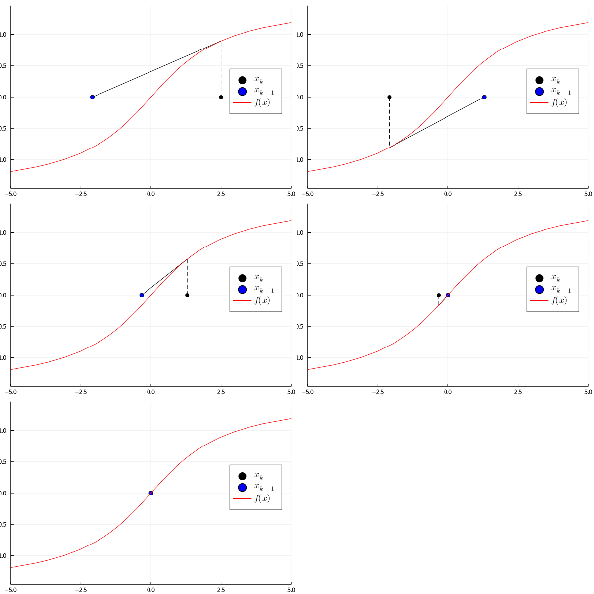
Let us demonstrate this with a simple example suppose we want to find the root of the function $f(x) = atan(\frac{x}{2})$ using $x_0=2.5$ as initial guess. The following animation shows the Newton method in action. Note that the derivative can be computed using the ForwardDiff package

f(x) = atan(x/2)
x0 = 2.5
y0 = f(x0)
d(f, x) = ForwardDiff.derivative(f, x)

xk = 2.5
yk = f(xk)

anim = @animate for i in 1:5
    xnew = xk - yk/d(f, xk)
    ynew = f(xnew)
    scatter([xk], [0]; markersize=5, markershape=:circle, c=:black, label="\$ x_k\$")
    plot!([xk, xk], [0, yk], linestyle=:dash, color=:black, label=nothing)
    plot!([xnew, xk], [0, yk], color=:black, label=nothing)
    scatter!([xnew], [0], color=:blue, markersize=5, label="\$x_{k+1}\$")
    plot!(f, -10, 10, label="\$f(x)\$", c=:red, legend=:right, legendfont=12, xlims=(-5, 5))
    global xk, yk = xnew, ynew
end

@show xk, yk

(xk, yk) = (-3.911818029136288e-8, -1.9559090145681437e-8)

After $5$ iterations the absolute error is already in the magnitude $10^{-8}$. If the initial guess $x_0$ is close enough to the correct root, then the Newton method can give a fast and accurate solution. However, it has no information about the error. This motives to find a generalized interval version.

Interval Newton method in 1D

Suppose we want to find the roots of a function $f$ over the interval $X$. Let us take as initial guess the the midpoint of $X$ $m(X)$. The core idea is now to consider all possible slopes a tangent line to $f$ in $X$ can have, instead of just the tangent at $m(X)$. This means we define the Newton operator

where $f'(X)$ takes into acount all possible slopes the tangent can have in $X$. As an example, consider the function $f(x)=atan(\frac{x}{2})$ with starting interval $X=[-1,5]$. Observe the following figure

X = -1..5
N(f, X) = mid(X) - f(mid(X))/d(f, X)
X = -1..5

Nx = N(f, X)
Xnext = Nx ∩ X

x0 = mid(X)
y0 = f(x0)
offset = 5e-2
plot([X.lo, X.hi], [-offset, -offset], label="\$X\$", c=:green, lw=2)
scatter!([x0], [-offset]; markersize=5, markershape=:circle, c=:black, label=nothing)
plot!([x0, x0], [-offset, y0], linestyle=:dash, color=:black, label=nothing)

deriv = d(f, X)
for m in range(deriv.lo, deriv.hi, length=100) # plot cone
    plot!([x0-y0/m, x0], [offset, y0], color=:gray, label=nothing, alpha=0.5)
end
plot!([Nx.lo, Nx.hi], [offset, offset], label="\$N(X)\$", c=:blue, lw=2)
plot!([Xnext.lo, Xnext.hi], [0, 0], label="\$N(x) \\cap X\$", c=:black, lw=3)
plot!(f, -10, 10, label="\$f(x)\$", c=:red, legend=:right)
plot!(legend=:bottomright, legendfont=12)

The green interval represents our starting interval. The gray area is the cone containing all lines passing through (m(X), f(m(X))) with slope in $f'(X)$. The blue interval is $N_f(X)$. Now, since we new the root has to been contained both in $X$ and in $N_f(X)$, we can conclude that the root must lie in $X \cap N_f(X)$, which is highlighted in dark in the figure. As you can notice, we squeezed the starting interval to a smaller one, which is guaranteed to contain the root. We are now ready to present the iteration of the interval newton method

Now the following important theorem holds

Theorem if $0 \notin f'(X)$, then the intervals $X_k$ form a nested sequence squeezing quadratically to the root of $f$.

Note that the condition $0 \notin f'(X)$ implies that either $f$ has a unique root in $X$ or no roots at all. An equivalent expression for this theorem is the following:

• If $N_f(X)\subseteq X$, then $X$ has a unique root

• if $N_f(X)\cap X=\emptyset$, then $f$ has no root in $X$.

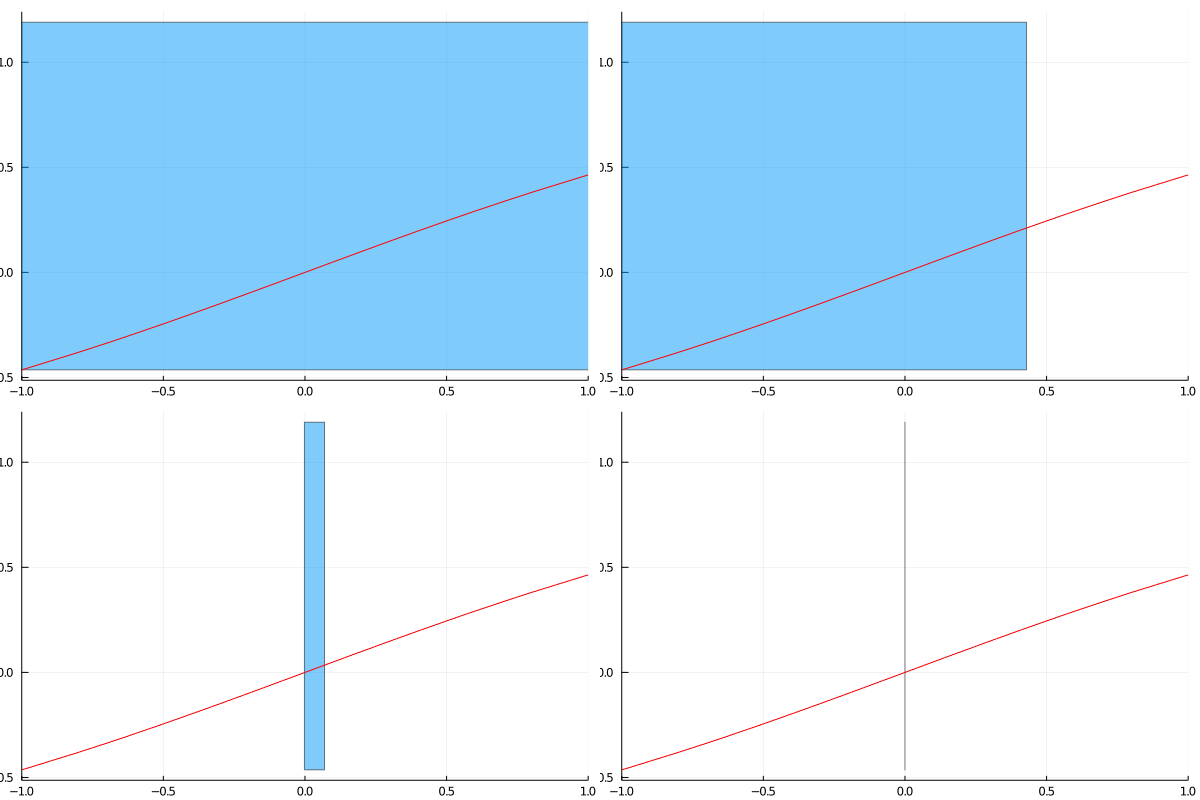
The following animation shows the Newton method in action with our example from before

function newton_iteration(f, df, X)
    m = @interval mid(X)
    return (m - f(m)/df(X)) ∩ X
end

xk = X
df(x) = d(f, x)
anim = @animate for i in 1:4
    zerobox = IntervalBox(xk, f(X))
    plot(zerobox)
    plot!(f, -1, 1, c=:red, xlims=(-1,1), legend=nothing)
    global xk = newton_iteration(f, df, xk)
    @show xk
end

xk = [-1, 0.4292036733]
xk = [-0.001913860913, 0.06895721471]
xk = [-3.670747462e-05, 3.138504583e-06]
xk = [-3.940431152e-16, 5.259983123e-15]

As you can see, after only $4$ iterations the interval has already shrunk to an interval of width $10^{-15}$, which is guaranteed to contain the true value of the root.

We have seen that the Newton method is very powerful when $0\notin f'(X)$, but what if this condition is not met? If $0\in f'(X)$, then division by zero occurs. This means that using traditional interval arithmetic the ratio $\frac{f(m(X))}{f'(X)}$ will be $[-\infty, \infty]$, which is not very useful. To overcome this problem we exploit extended division, suppose $0\in f'(X_k)=Y=[\underline{Y}, \overline{Y}]$, then we consider the two intervals $Y_1=[\underline{Y},0]$ and $Y_2=[0,\overline{Y}]$. Then we apply the update formula using both intervals obtaining the two intervals

and then repeat Newton iteration with extended division to both interals. Hence, in the worst-case scenario we will double the number of intervals to track. If at some point we have $X_k=\emptyset$, then we can conclude it has no roots and it can bo thrown away. If $N_f(X_k)\subseteq X_k$, then the root is unique and we do not need to split the interval with extended division anymore.

Generalization to higher dimensions

The Interval Newton method can be generalized to higher dimensions replacing the derivative with the Jacobian. Suppose you want to solve the system $F(\mathbf{x})=\mathbf{0}$, where $F:\mathbb{R}^n\rightarrow\mathbb{R}^n$. Now the update formula for interval Newton is

where $X_k$ is now an interval box.