Interval constraint programming tutorial

Download the notebook for this tutorial.

Setup

The IntervalConstraintProgramming.jl package can be installed with

julia> using Pkg; Pkg.add("IntervalConstraintProgramming")

Once the package is installed, it can be imported. Note that you will need also the IntervalArithmetic.jl package.

using IntervalArithmetic, IntervalConstraintProgramming

Introduction

Given a domain $X$ and a set of constraint $S$, constraint programming aims to determine all points in the domain $X$ that satisfy the constraint $S$.

This Julia package allows you to specify a set of constraints on real-valued variables, given by (in)equalities, and rigorously calculate inner and outer approximations to the feasible set, i.e. the set that satisfies the constraints. This uses interval arithmetic provided by the IntervalArithmetic.jl package, in particular multi-dimensional IntervalBoxes, i.e. Cartesian products of one-dimensional intervals.

Basic usage

The simple way to define a constraint is to use the @constraint macro, as the following example demonstrates

S = @constraint x^2 + y^2 <= 1

Separator:
  - variables: x, y
  - expression: x ^ 2 + y ^ 2 ∈ [-∞, 1]

As it can be noticed, the macro itself can figure out that $x$ and $y$ are variables and you do not need to define those separately. The output of the macro is an object of type Separator. To understand what it means, we first need to introduce a few terms.

• Inner contractor: The smallest box containing all points in the domain $X$ that satisfy the constraint $S$.

• Outer contractor: The smallest box containing all points in the domain $X$ that do not satisfy the constraint $S$.

The separator is now simply a function that returns the inner and outer contractor when applied to a domain. The domain should have always type IntervalBox, even when it is a 1-dimensional box (i.e. an interval). Let us look an example on how to get an inner and outer contractor.

X = IntervalBox(-100..100, 2)

inner, outer = S(X)

@show inner

@show outer

inner = [-1, 1] × [-1, 1]
outer = [-100, 100] × [-100, 100]

Note Points on the boundary are counted both as inner and outer points. In other words if our constraint is e.g. $x\leq1$, then the inner contractor will be the smallest box containing all points in the domain that satisfy $x\leq 1$ and the outer contractor all points satisfying $x\geq1$. Not that the equality is kept in both inequalities. To better understand this, consider the following example: let us look for the points in the real line $\mathbb{R}$ satisfying $-1\leq x\leq0$, using $X=[-1,1]$ as domain. The "pen and paper" solution would be that $[-1,0]$ is the inner contractor and $]0,1]$ is the outer contractor. However, we get the following result:

S = @constraint -1<=x<=0
X = IntervalBox(-1..1, 1)

@show inner, outer = S(X)

(inner, outer) = S(X) = ([-1, 0], [-1, 1])

The inner contractor is what we expected. For the outer contractor, the key point is that the negation of $-1\leq x\leq 0$ is $x\leq-1 \cup x\geq 0$. I.e. the outer contractor looks for the smallest box inside the domain $[-1,1]$ which satisfies $x\leq-1 \cup x\geq 0$. This is the smallest box containing $-1$ and $[0, 1]$, i.e. the whole domain $[-1, 1]$. Let us take another example with the same constraint but a different domain

X = IntervalBox(-0.5..0.5, 1)
@show inner, outer = S(X)

(inner, outer) = S(X) = ([-0.5, 0], [0, 0.5])

Now the outer contractor looks for the point inside $[-0.5, 0.5]$ satisfying $x\leq-1 \cup x\geq 0$, i.e $[0, 0.5]$.

First application: set inversion

Given a function $f:\R^m\rightarrow\R^n$ and a set $Y\subset\R^n$, set inversion means to find the set $X=f^{-1}(Y)=\{x\in\R^m|f(x)\in Y\}$, which is refered as feasible set. Generally, the image set Y can be represented as a set of constraints on the expression $f(X)$ and solving the set inversion problem means to find the points in $X$ for which these constraints are satisfied. As we show in this example, set inversion can be solved using interval constraint programming. Let's consider the function $f(x, y) = x^2+y^2$ and let's find the set $X$ for which $f(X)\in[1, 3]$, i.e. we must find the points $(x, y)$ for which $1\leq x^2+y^2\leq 3$. Let's define this constraint

S = @constraint 1 <= x^2+y^2 <= 3

Separator:
  - variables: x, y
  - expression: x ^ 2 + y ^ 2 ∈ [1, 3]

The strategy to solve this problem is the following, we start with a large interval box, which we know will contain the feasible sets and we iteratively divide the box in smaller boxes, keeping track of which boxes are guaranteed to be inside the feasible sets, the boxes that are outside and the boxes that are on the boundary. IntervalConstraintProgramming offers the function pave, to do so, the signature of this function is

pave(S, X, tol)

where $S$ is our Separator, $X$ is our starting box and $tol$ is a tolerance parameter. This function returns an object of type SubPaving, which stores a list of boxes guaranteed to be into the feasible set in the attribute inner, as well as a list of boxes on the boundary in the attribute boundary.

X = IntervalBox(-100..100, 2) # our starting box
paving = pave(S, X, 0.125)

Paving:
- tolerance ϵ = 0.125
- inner approx. of length 164
- boundary approx. of length 164

As we can see, the function found in total 164 boxes inside the feasible set and 164 boxes at the boundary. We can now visualize how well paving approximates the feasible set

using Plots
plot(paving.inner, c="green", aspect_ratio=:equal, label="inner")
plot!(paving.boundary, c="gray", label="boundary")

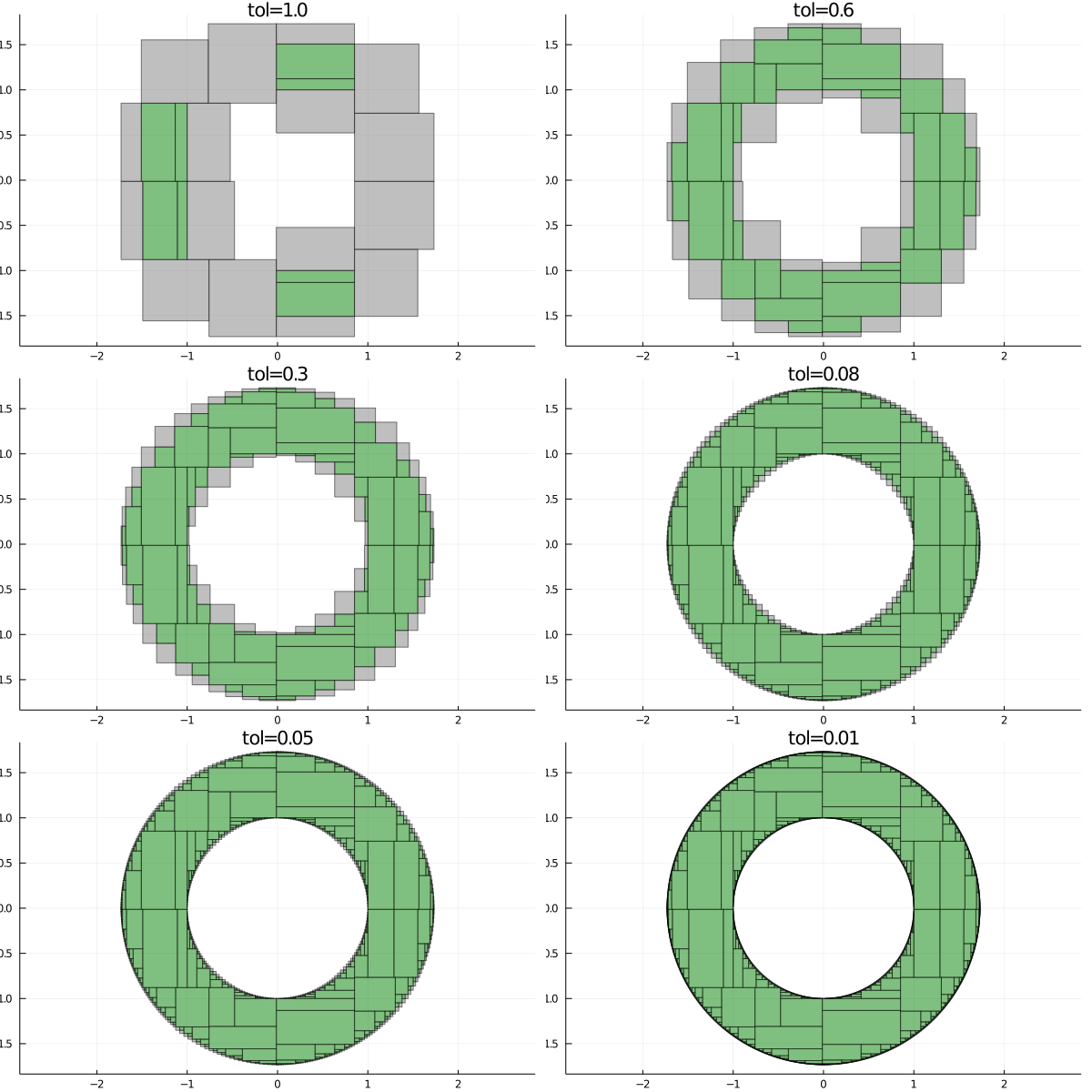
The smallest the tolerance parameter, the better the approximation of the feasible set will be, as the following animation shows

tolerances =  append!(collect(1:-0.1:0.1), collect(0.09:-0.01:0.01))
anim = @animate for tol in tolerances
    paving = pave(S, X, tol)
    plot(paving.inner, c="green", legend=false, title="tol=$tol", aspect_ratio=:equal)
    plot!(paving.boundary, c="gray")
end

Constraint Programming with ModelingToolkit

The @constraint macro is very handy, but it can handle only simple expressions. If you want to handle more complicated expressions, you can use IntervalConstraintProgramming with ModelingToolkit. The following example shows how to import the package and define variables

using ModelingToolkit
vars = @variables x y

(x, y)

Once you have defined the variables, you can construct a separator using the Separator constructor, which take an array of variables as first parameter and a function representing the constraint as second parameter, observe

f(x, y) = x + y < 3

S = Separator(vars, f)

Separator:
  - variables: x, y
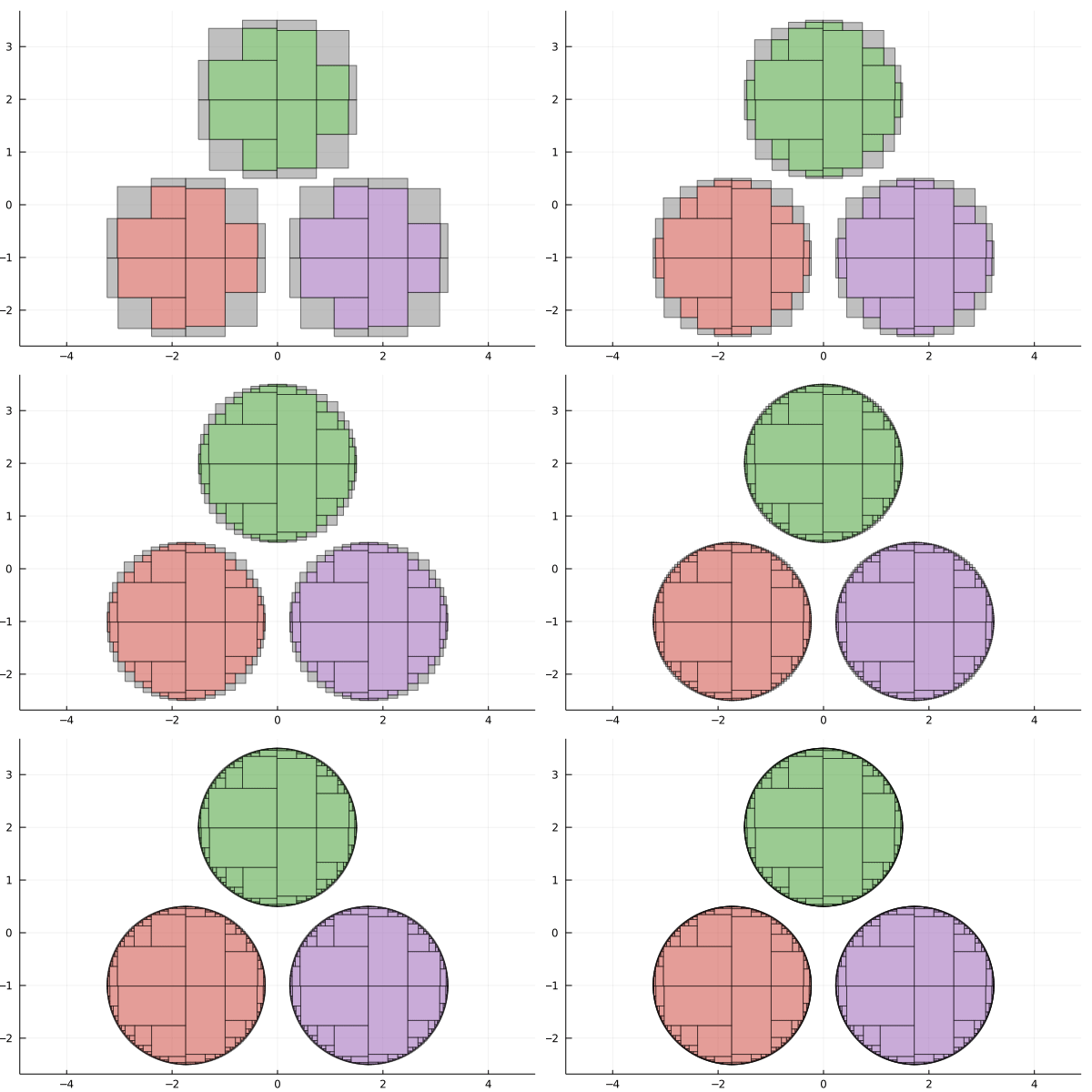
  - expression: x + y == [-∞, 3]

After that, you can use the separator and the pave function as described before. As an example, let us draw the Julia logo solving a set inversion problem. We have already defined the variables, now the equations of the 3 circles are

circle1(x, y) = (x + √3)^2 + (y + 1)^2 - 9/4 < 0
circle2(x, y) = (x - √3)^2 + (y + 1)^2 - 9/4 < 0
circle3(x, y) = x^2 + (y - 2)^2 - 9/4 < 0

circle3 (generic function with 1 method)

Now we can define the corresponding separators.

S1 = Separator(vars, circle1)
S2 = Separator(vars, circle2)
S3 = Separator(vars, circle3)

Separator:
  - variables: x, y
  - expression: (x ^ 2 + (y - 2) ^ 2) - 2.25 == [-∞, 0]

Now we can use pave with diferent tolerances to plot the Julia logo

X = IntervalBox(-4..4, 2)
anim = @animate for tol in 2.0 .^ (0:-1:-6)
    paving1 = pave(S1, X, tol)
    paving2 = pave(S2, X, tol)
    paving3 = pave(S3, X, tol)
    plot(legend=false, aspect_ratio=:equal)

    plot!(paving1.boundary, color=:gray, alpha=0.5)
    plot!(paving2.boundary, color=:gray, alpha=0.5)
    plot!(paving3.boundary, color=:gray, alpha=0.5)

    plot!(paving1.inner, color=RGB(0.796, 0.235, 0.2))
    plot!(paving2.inner, color=RGB(0.584, 0.345, 0.698))
    plot!(paving3.inner, color=RGB(0.22, 0.596, 0.149))
end