Preconditioning interval linear systems

Preconditioning interval linear systems

Basic concepts

Consider the square interval linear system

\[\mathbf{Ax}=\mathbf{b},\]

preconditioning the interval linear system by a real matrix $C$ means to multiply both sides of the equation by $C$, obtaining the new system

\[C\mathbf{Ax}=C\mathbf{b},\]

which is called preconditioned system. Let us denote by $A_c$ the midpoint matrix of $\mathbf{A}$. Popular choices for $C$ are

Inverse midpoint preconditioning: $C\approx A_c^{-1}$
Inverse diagonal midpoint preconditioning: $C\approx D_{A_c}^{-1}$ where $D_{A_c}$ is the diagonal matrix containing the main diagonal of $A_c$.

Advantages of preconditioning

Using preconditioning to solve an interval linear system can have mainly two advantages.

Extend usability of algorithms

Some algorithms require the matrix to have a specific structure in order to be used. For example Hansen-Bliek-Rohn algorithm requires $\mathbf{A}$ to be an H-matrix. However, the algorithm can be extended to work to strongly regular matrices using inverse midpoint preconditioning. (Recall that an interval matrix is strongly regular if $A_c^{-1}\mathbf{A}$ is an H-matrix).

Improve numerical stability

Even if the algorithms theoretically work, they can be prone to numerical instability without preconditioning. This is demonstrated with the following example, a more deep theoretical analysis can be found in [NEU90].

Let $\mathbf{A}$ be an interval lower triangular matrix with all $[1, 1]$ in the lower part, for example

using IntervalLinearAlgebra

N = 5 # problem dimension
A = tril(fill(1..1, N, N))

5×5 Matrix{Interval{Float64}}:
 [1, 1]  [0, 0]  [0, 0]  [0, 0]  [0, 0]
 [1, 1]  [1, 1]  [0, 0]  [0, 0]  [0, 0]
 [1, 1]  [1, 1]  [1, 1]  [0, 0]  [0, 0]
 [1, 1]  [1, 1]  [1, 1]  [1, 1]  [0, 0]
 [1, 1]  [1, 1]  [1, 1]  [1, 1]  [1, 1]

and let $\mathbf{b}$ having $[-2, 2]$ as first element and all other elements set to zero

b = vcat(-2..2, fill(0, N-1))

5-element Vector{Interval{Float64}}:
 [-2, 2]
  [0, 0]
  [0, 0]
  [0, 0]
  [0, 0]

the "pen and paper" solution would be $[[-2, 2], [-2, 2], [0, 0], [0, 0], [0, 0]]^\mathsf{T}$, that is a vector with $[-2, 2]$ as first two elements and all other elements set to zero. Now, let us try to solve without preconditioning.

solve(A, b, GaussianElimination(), NoPrecondition())

5-element Vector{Interval{Float64}}:
   [-2, 2]
   [-2, 2]
   [-4, 4]
   [-8, 8]
 [-16, 16]

solve(A, b, HansenBliekRohn(), NoPrecondition())

5-element Vector{Interval{Float64}}:
   [-2, 2]
   [-2, 2]
   [-4, 4]
   [-8, 8]
 [-16, 16]

It can be seen that the width of the intervals grows exponentially, this gets worse with bigger matrices.

N = 100 # problem dimension
A1 = tril(fill(1..1, N, N))
b1 = [-2..2, fill(0..0, N-1)...]

solve(A1, b1, GaussianElimination(), NoPrecondition())

100-element Vector{Interval{Float64}}:
     [-2, 2]
     [-2, 2]
     [-4, 4]
     [-8, 8]
   [-16, 16]
   [-32, 32]
   [-64, 64]
 [-128, 128]
 [-256, 256]
 [-512, 512]
           ⋮
         [-2.47589e+27, 2.47589e+27]
         [-4.95177e+27, 4.95177e+27]
         [-9.90353e+27, 9.90353e+27]
         [-1.98071e+28, 1.98071e+28]
         [-3.96141e+28, 3.96141e+28]
         [-7.92282e+28, 7.92282e+28]
         [-1.58457e+29, 1.58457e+29]
         [-3.16913e+29, 3.16913e+29]
         [-6.33826e+29, 6.33826e+29]

solve(A1, b1, HansenBliekRohn(), NoPrecondition())

100-element Vector{Interval{Float64}}:
     [-2, 2]
     [-2, 2]
     [-4, 4]
     [-8, 8]
   [-16, 16]
   [-32, 32]
   [-64, 64]
 [-128, 128]
 [-256, 256]
 [-512, 512]
           ⋮
         [-2.47589e+27, 2.47589e+27]
         [-4.95177e+27, 4.95177e+27]
         [-9.90353e+27, 9.90353e+27]
         [-1.98071e+28, 1.98071e+28]
         [-3.96141e+28, 3.96141e+28]
         [-7.92282e+28, 7.92282e+28]
         [-1.58457e+29, 1.58457e+29]
         [-3.16913e+29, 3.16913e+29]
         [-6.33826e+29, 6.33826e+29]

However this numerical stability issue is solved using inverse midpoint preconditioning.

solve(A, b, GaussianElimination(), InverseMidpoint())

5-element Vector{Interval{Float64}}:
 [-2, 2]
 [-2, 2]
  [0, 0]
  [0, 0]
  [0, 0]

solve(A, b, HansenBliekRohn(), InverseMidpoint())

5-element Vector{Interval{Float64}}:
 [-2, 2]
 [-2, 2]
  [0, 0]
  [0, 0]
  [0, 0]

Disadvantages of preconditioning

While preconditioning is useful, sometimes even necessary, to solve interval linear systems, it comes at a price. It is important to understand that the preconditioned interval linear system is not equivalent to the original one, particularly the preconditioned problem can have a larger solution set.

Let us consider the following linear system

A = [2..4 -2..1;-1..2 2..4]

2×2 Matrix{Interval{Float64}}:
  [2, 4]  [-2, 1]
 [-1, 2]   [2, 4]

b = [-2..2, -2..2]

2-element Vector{Interval{Float64}}:
 [-2, 2]
 [-2, 2]

Now we plot the solution set of the original and preconditioned problem using Oettli-Präger

using LazySets, Plots

polytopes = solve(A, b, LinearOettliPrager())
polytopes_precondition = solve(A, b, LinearOettliPrager(), InverseMidpoint())

plot(UnionSetArray(polytopes_precondition), ratio=1, label="preconditioned", legend=:right)
plot!(UnionSetArray(polytopes), label="original", α=1)
xlabel!("x")
ylabel!("y")

"/home/runner/work/IntervalLinearAlgebra.jl/IntervalLinearAlgebra.jl/docs/build/explanations/solution_set_precondition.png"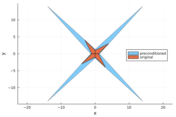

Take-home lessons

Preconditioning an interval linear system can enlarge the solution set
Preconditioning is sometimes needed to achieve numerical stability
A rough rule of thumb (same used by IntervalLinearAlgebra.jl if no preconditioning is specified)
- not needed for M-matrices and strictly diagonal dominant matrices
- might be needed for H-matrices (IntervalLinearAlgebra.jl uses inverse midpoint by default with H-matrices)
- must be used for strongly regular matrices