Taylor models tutorial

Download the notebook for this tutorial.

Setup

The TaylorModels.jl package can be installed with

julia> using Pkg; Pkg.add("TaylorModels")

Once the package is installed, it can be imported. Note that you will need also the IntervalArithmetic.jl package.

using IntervalArithmetic, TaylorModels

Introduction

Given a function $f$ which is continuously derivable $n+1$ times, its nth-order taylor approximation around the point $x_0$ is given by

where $P_n(x)$ is a polynomial of degree $n$. It is well known that Taylor expansion gives a good approximation in a small neighbourhood around $x_0$. However it does not give any information on the approximation error.

TaylorModels.jl uses interval arithmetic to give a rigorous polynomial approximation of $f$ over the interval $[a, b]$. More formally, the rigorous approximation is given by the pair $(P_n(x), \Delta)$, where

• $P_n(x)$ is a polynomial of degree $n$, whose coefficients are intervals.

• $\Delta$ is the interval remainder, and it provides an estimate of all numerical errors (rounding, truncation) encoutered during Taylor expansion computation, i.e. it is guaranteed that $\forall x\in[a, b]:~|P(x)-f(x)|\in\Delta$.

Taylor models for univariate function

Let us now describe how to get the rigorous Taylor approximation for a function $f$ in an interval $a$ around the point $x_0$. Let us define our parameters

f(x) = x*(x-1.1)*(x+2)*(x+2.2)*(x+2.5)*(x+3)*sin(1.7*x+0.5)
a = -0.5..1
x0 = mid(a) # expansion around the middle point of the domain

0.25

To create a Taylor model of order $n$ in the interval $a$ around the point $x_0$ we need the function TaylorModel1 from TaylorModels.jl, (note the 1 stands for 1 dimensional). The signature of this function is Note that x_0 must be given as an interval, even though it is a single point. Observe the following example, where we create a Taylor approximation of order 6 and 7

tm6 = TaylorModel1(6, interval(x0), a)
tm7 = TaylorModel1(7, interval(x0), a)
@show tm6
@show tm7

tm6 =  [0.25, 0.25] + [1, 1] t + [0, 0]
tm7 =  [0.25, 0.25] + [1, 1] t + [0, 0]

Now to compute the Taylor approximation of our functions we can simply give the previously constructed Taylor model to the function as input

ftm6 = f(tm6)
ftm7 = f(tm7)
@show ftm6
@show ftm7

ftm6 =  [-8.36112, -8.36111] + [-47.0612, -47.0611] t + [-38.3545, -38.3544] t² + [90.4376, 90.4377] t³ + [102.183, 102.184] t⁴ + [-20.5814, -20.5813] t⁵ + [-58.0084, -58.0083] t⁶ + [-1.97165, 2.71142]
ftm7 =  [-8.36112, -8.36111] + [-47.0612, -47.0611] t + [-38.3545, -38.3544] t² + [90.4376, 90.4377] t³ + [102.183, 102.184] t⁴ + [-20.5814, -20.5813] t⁵ + [-58.0084, -58.0083] t⁶ + [-14.3341, -14.334] t⁷ + [-0.281401, 1.03908]

The last term of the expression is the interval remainder and the previous ones represent the Taylor polynomial. The result is an object of type TaylorModel1 with the following attributes

• dom: inverval over which the Taylor approximation is computed ($a$ in our example)

• pol: polynomial approximation of the function

• rem: interval remainder

• x0: center of Taylor expansion ($x_0$ in our example)

Now we can visualize how well our taylor model works using the plot function.

using Plots
plot(range(inf(a), stop=sup(a), length=1000), f, lw=2, xaxis="x", yaxis="f(x)", label="f(x)")
plot!(ftm6, label="6th order")
plot!(ftm7, label="7th order")

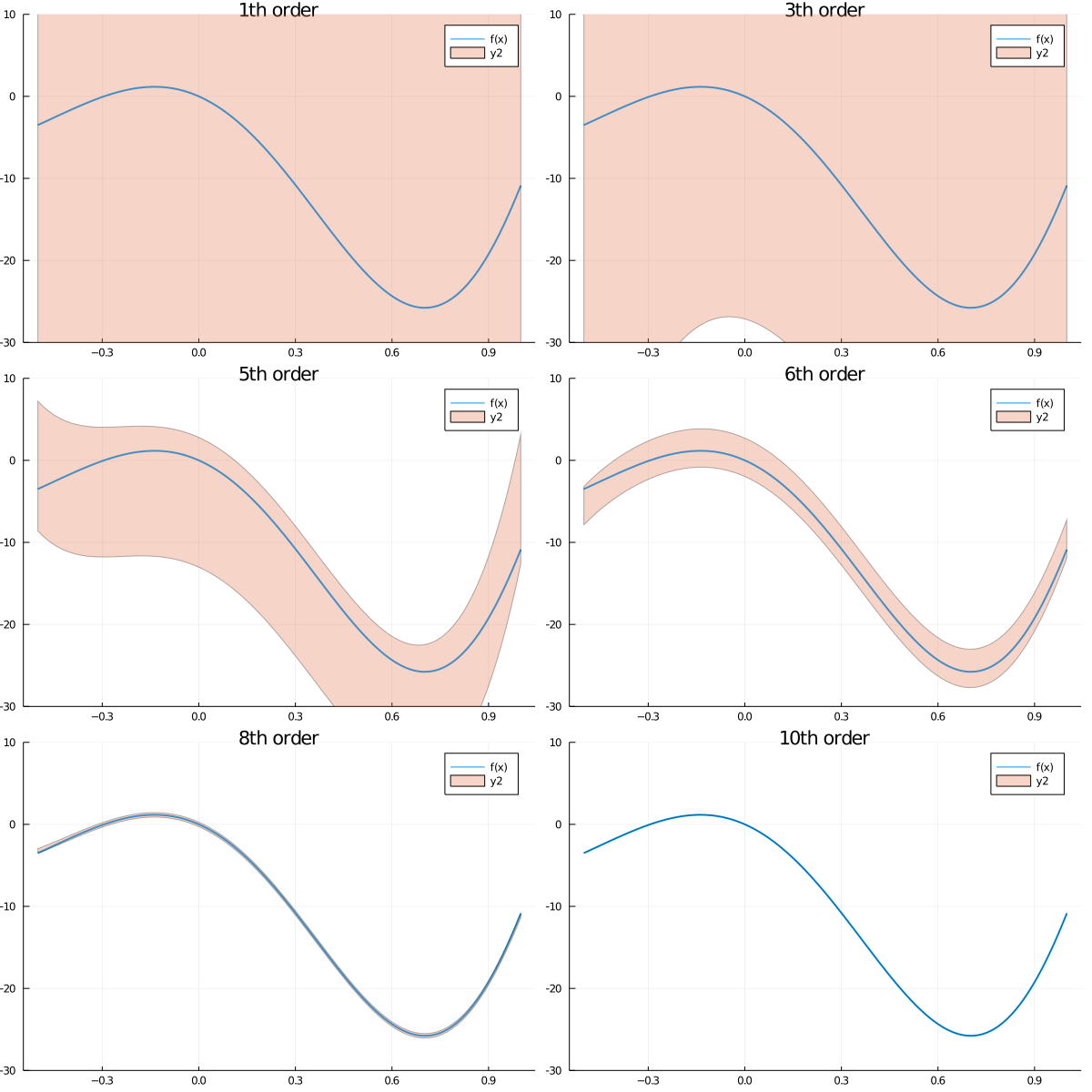
As you can notice, the Taylor model produces a "band" around the function and the polynomial approximation is guaranteed to be somewhere inside that bar. As you may expect, the higher the order of the model, the narrower the band will be, as the following animation shows

orders = [1, 2, 3, 4, 5, 6, 7, 8, 9, 10]
anim = @animate for n in orders
    tm = TaylorModel1(n, interval(x0), a)
    ftm = f(tm)
    plot(range(inf(a), stop=sup(a), length=1000), f, lw=2, xaxis="x", yaxis="f(x)",
         label="f(x)", ylims=(-30, 10))
    plot!(ftm, title="$(n)th order")
end